838 CHAPTER 39. STATISTICAL TESTS

the number of unknown parameters and to replace each parameter with its maximum like-lihood estimate. The proof of this is very technical and you can see it discussed in Cramér,[9].

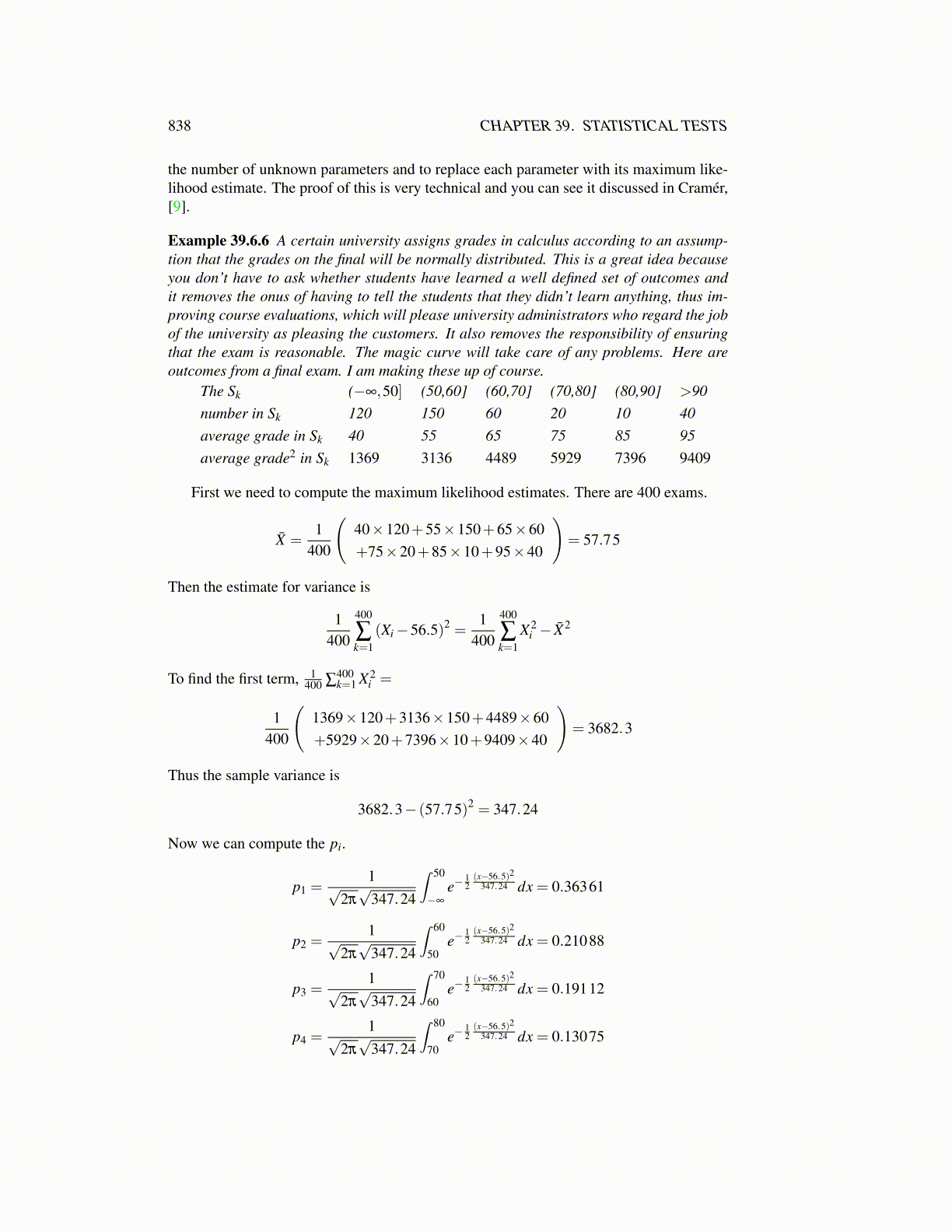
Example 39.6.6 A certain university assigns grades in calculus according to an assump-tion that the grades on the final will be normally distributed. This is a great idea becauseyou don’t have to ask whether students have learned a well defined set of outcomes andit removes the onus of having to tell the students that they didn’t learn anything, thus im-proving course evaluations, which will please university administrators who regard the jobof the university as pleasing the customers. It also removes the responsibility of ensuringthat the exam is reasonable. The magic curve will take care of any problems. Here areoutcomes from a final exam. I am making these up of course.

The Sk (−∞,50] (50,60] (60,70] (70,80] (80,90] >90number in Sk 120 150 60 20 10 40average grade in Sk 40 55 65 75 85 95average grade2 in Sk 1369 3136 4489 5929 7396 9409

First we need to compute the maximum likelihood estimates. There are 400 exams.

X̄ =1

400

(40×120+55×150+65×60+75×20+85×10+95×40

)= 57.75

Then the estimate for variance is

1400

400

∑k=1

(Xi−56.5)2 =1

400

400

∑k=1

X2i − X̄2

To find the first term, 1400 ∑

400k=1 X2

i =

1400

(1369×120+3136×150+4489×60+5929×20+7396×10+9409×40

)= 3682.3

Thus the sample variance is

3682.3− (57.75)2 = 347.24

Now we can compute the pi.

p1 =1√

2π√

347.24

∫ 50

−∞

e−12(x−56.5)2

347.24 dx = 0.36361

p2 =1√

2π√

347.24

∫ 60

50e−

12(x−56.5)2

347.24 dx = 0.21088

p3 =1√

2π√

347.24

∫ 70

60e−

12(x−56.5)2

347.24 dx = 0.19112

p4 =1√

2π√

347.24

∫ 80

70e−

12(x−56.5)2

347.24 dx = 0.13075