39.6. GOODNESS OF FIT 837

Actually, there is a fly in the ointment. You know the random variable is not exactlyX 2 (5). After all, you only used a sample of 60 = n. The idea is to let n→ ∞. Cramérsays that if n is large enough that the expected numbers npi ≥ 10 for each Si, then theapproximation will be good enough for ordinary applications. Of course you end up beingmore sure if you take n larger. More information is typically better.

This process illustrates another example of Hypothesis testing. In this case, the “nullhypothesis” is that the die is fair and the density function is 1/6 for each outcome. Theabove process indicates that we should reject the “null hypothesis” with probability .98.This is a general notion in statistics called hypothesis testing. There is quite a bit of jargonassociated with this, but the main idea is illustrated by the above example. Here is anotherexample where it is not so clear.

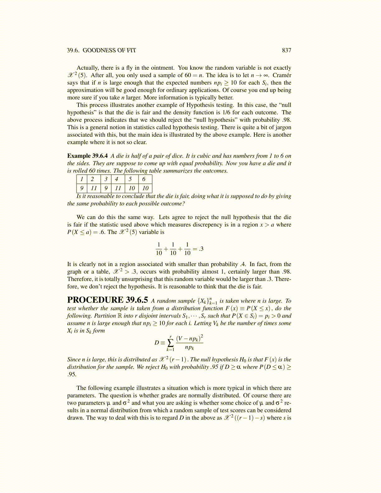
Example 39.6.4 A die is half of a pair of dice. It is cubic and has numbers from 1 to 6 onthe sides. They are suppose to come up with equal probability. Now you have a die and itis rolled 60 times. The following table summarizes the outcomes.

1 2 3 4 5 69 11 9 11 10 10

Is it reasonable to conclude that the die is fair, doing what it is supposed to do by givingthe same probability to each possible outcome?

We can do this the same way. Lets agree to reject the null hypothesis that the dieis fair if the statistic used above which measures discrepency is in a region x > a whereP(X ≤ a) = .6. The X 2 (5) variable is

110

+1

10+

110

= .3

It is clearly not in a region associated with smaller than probability .4. In fact, from thegraph or a table, X 2 > .3, occurs with probability almost 1, certainly larger than .98.Therefore, it is totally unsurprising that this random variable would be larger than .3. There-fore, we don’t reject the hypothesis. It is reasonable to think that the die is fair.

PROCEDURE 39.6.5 A random sample {Xk}nk=1 is taken where n is large. To

test whether the sample is taken from a distribution function F (x) ≡ P(X ≤ x) , do thefollowing. Partition R into r disjoint intervals S1, · · · ,Sr such that P(X ∈ Si) = pi > 0 andassume n is large enough that npi ≥ 10 for each i. Letting Vk be the number of times someXi is in Sk form

D≡r

∑k=1

(V −npk)2

npk

Since n is large, this is distributed as X 2 (r−1) . The null hypothesis H0 is that F (x) is thedistribution for the sample. We reject H0 with probability .95 if D≥ α where P(D≤ α)≥.95.

The following example illustrates a situation which is more typical in which there areparameters. The question is whether grades are normally distributed. Of course there aretwo parameters µ and σ2 and what you are asking is whether some choice of µ and σ2 re-sults in a normal distribution from which a random sample of test scores can be considereddrawn. The way to deal with this is to regard D in the above as X 2 ((r−1)− s) where s is