826 CHAPTER 39. STATISTICAL TESTS

Should the above condition be assumed? I am not sure, from the point of view ofrigorous math, but this kind of thing is often assumed in experimental work and leads touseful conclusions and is not unreasonable since it is just an assumption that the randomvariables for each ti are normally distributed.

For example suppose someone is developing vaccines for antiplasmosis, a disease inanimals which causes anemia. You can measure anemia easily by keeping track of thepacked cell volume. He has 15 animals which are infected by the disease and every week,he takes a small sample of blood from each and measures this packed cell volume using acentrifuge and capillary tubes. These measurements yield the Xk. If he had another groupof animals say 20 which have been given a vaccine, how would he tell if the vaccine waseffective? He would look for differences in the two different values of β . If he has a confi-dence interval for each β , the one for the vaccinated cows and the one for the unvaccinatedones, he could possibly conclude that his vaccine was working. An ordinary least squaresapproach would approximate the data with a straight line for each group of animals andwould give a slope β̂ based solely on geometric conditions. This may suggest that the vac-cine is working, but to be sure the pictures mean something, he needs a confidence intervalor something similar involving a probability for the two parameters β , not just the estimateβ̂ . It would of course also be very interesting to estimate the variance. The machinery fordoing these estimates will be considered in this section. It is a very nice application of theresults of the last section in which the distribution of quadratic forms was considered.

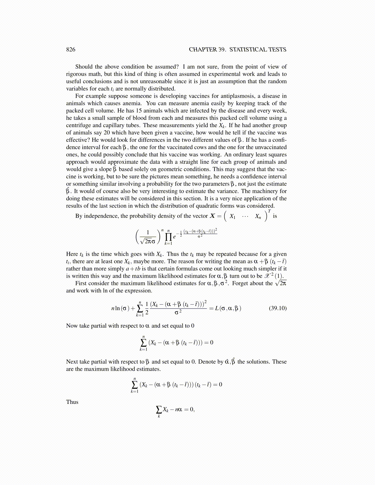
By independence, the probability density of the vector X =(

X1 · · · Xn

)Tis

(1√

2πσ

)n n

∏k=1

e−12(xk−(α+β(tk−t̄)))2

σ2

Here tk is the time which goes with Xk. Thus the tk may be repeated because for a giventi, there are at least one Xk, maybe more. The reason for writing the mean as α +β (tk− t̄)rather than more simply a+ tb is that certain formulas come out looking much simpler if itis written this way and the maximum likelihood estimates for α,β turn out to be X 2 (1).

First consider the maximum likelihood estimates for α,β ,σ2. Forget about the√

2π

and work with ln of the expression.

n ln(σ)+n

∑k=1

12(Xk− (α +β (tk− t̄)))2

σ2 = L(σ ,α,β ) (39.10)

Now take partial with respect to α and set equal to 0

n

∑k=1

(Xk− (α +β (tk− t̄))) = 0

Next take partial with respect to β and set equal to 0. Denote by α̂, β̂ the solutions. Theseare the maximum likelihood estimates.

n

∑k=1

(Xk− (α +β (tk− t̄)))(tk− t̄) = 0

Thus∑k

Xk−nα = 0,