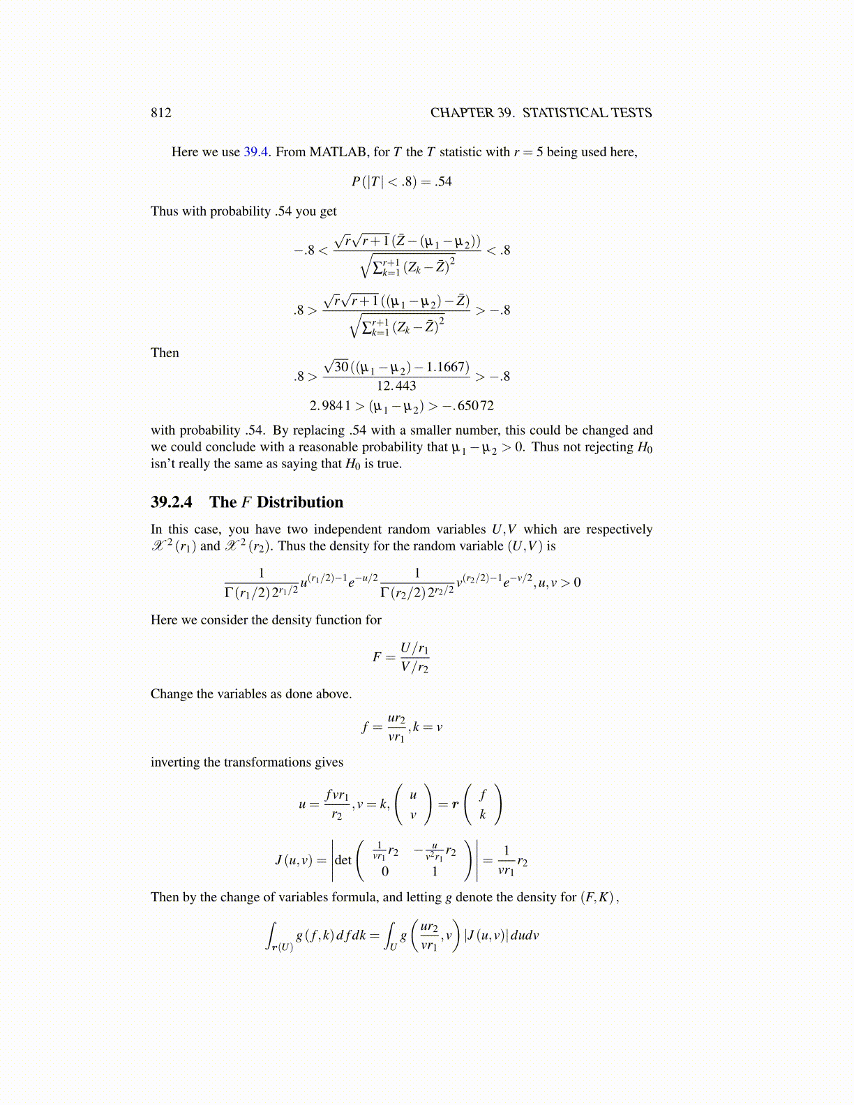
812 CHAPTER 39. STATISTICAL TESTS

Here we use 39.4. From MATLAB, for T the T statistic with r = 5 being used here,

P(|T |< .8) = .54

Thus with probability .54 you get

−.8 <

√r√

r+1(Z̄− (µ1−µ2))√∑

r+1k=1 (Zk− Z̄)2

< .8

.8 >

√r√

r+1((µ1−µ2)− Z̄)√∑

r+1k=1 (Zk− Z̄)2

>−.8

Then

.8 >

√30((µ1−µ2)−1.1667)

12.443>−.8

2.9841 > (µ1−µ2)>−.65072

with probability .54. By replacing .54 with a smaller number, this could be changed andwe could conclude with a reasonable probability that µ1− µ2 > 0. Thus not rejecting H0isn’t really the same as saying that H0 is true.

39.2.4 The F DistributionIn this case, you have two independent random variables U,V which are respectivelyX 2 (r1) and X 2 (r2). Thus the density for the random variable (U,V ) is

1Γ(r1/2)2r1/2 u(r1/2)−1e−u/2 1

Γ(r2/2)2r2/2 v(r2/2)−1e−v/2,u,v > 0

Here we consider the density function for

F =U/r1

V/r2

Change the variables as done above.

f =ur2

vr1,k = v

inverting the transformations gives

u =f vr1

r2,v = k,

(uv

)= r

(fk

)

J (u,v) =

∣∣∣∣∣det

(1

vr1r2 − u

v2r1r2

0 1

)∣∣∣∣∣= 1vr1

r2

Then by the change of variables formula, and letting g denote the density for (F,K) ,∫r(U)

g( f ,k)d f dk =∫

Ug(

ur2

vr1,v)|J (u,v)|dudv