798 CHAPTER 39. STATISTICAL TESTS

already been considered. The last two are described below.An interesting observation about all of this is that there is a gap between the theory and

the applications like those mentioned above. To really understand the mathematical theory,you need much more advanced mathematics than what is encountered in this book. Thishappens as soon as you start asking fundamental questions about what a random variableis independent of some application or why certain limits exist and in what sense they exist.Some of the most fundamental questions come from the Kolmogorov extension theoremwhich has to do with measures defined on infinite products.

39.1 The Distribution of nS2/σ2

In all of this, Xk is a random variable and we assume X1,X2, ... are independent. For ex-ample, you might have a large population of people and the weight of a person is normallydistributed. Then Xi would be the ith observation of a randomly selected person’s weight.

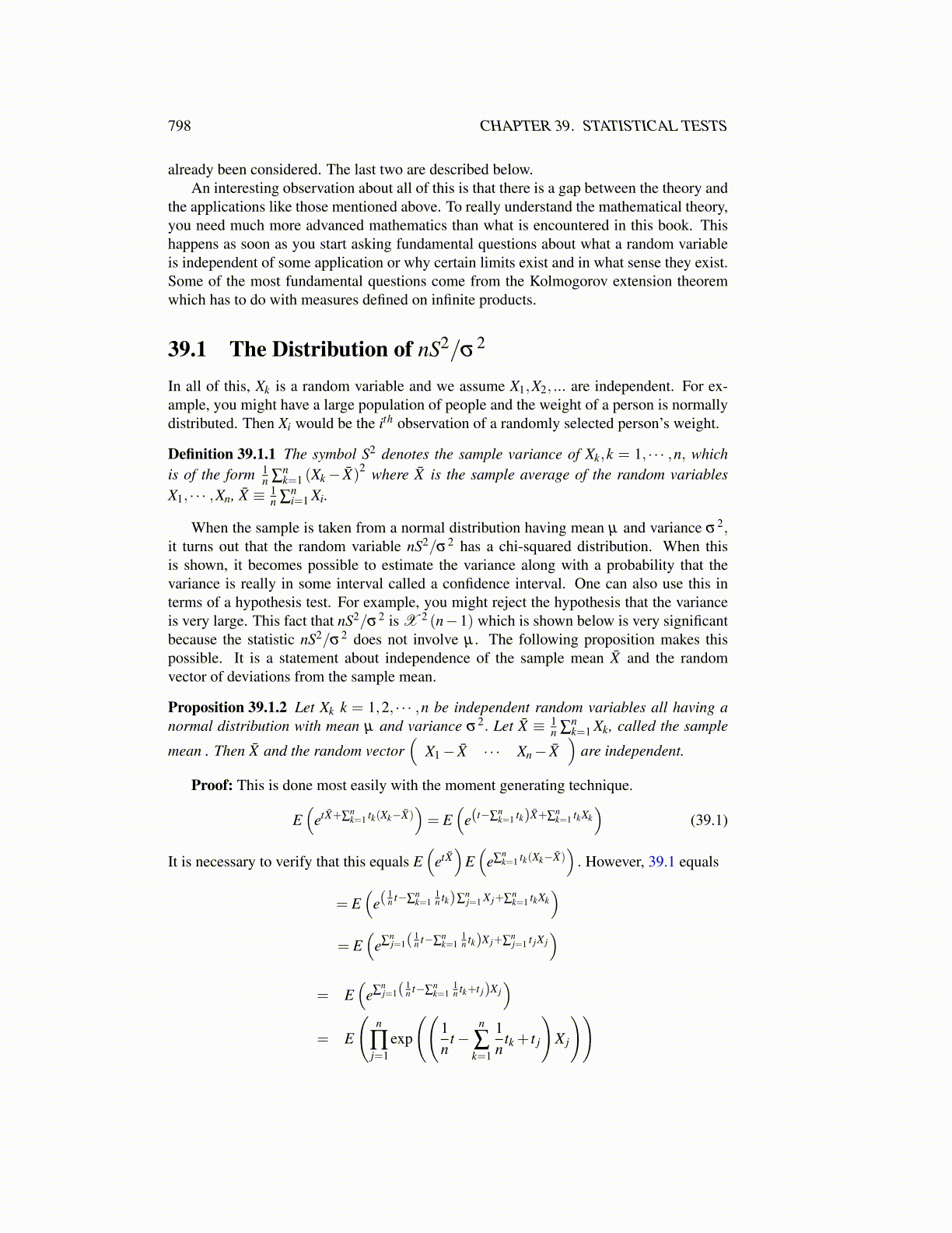
Definition 39.1.1 The symbol S2 denotes the sample variance of Xk,k = 1, · · · ,n, whichis of the form 1

n ∑nk=1 (Xk− X̄)

2 where X̄ is the sample average of the random variablesX1, · · · ,Xn, X̄ ≡ 1

n ∑ni=1 Xi.

When the sample is taken from a normal distribution having mean µ and variance σ2,it turns out that the random variable nS2/σ2 has a chi-squared distribution. When thisis shown, it becomes possible to estimate the variance along with a probability that thevariance is really in some interval called a confidence interval. One can also use this interms of a hypothesis test. For example, you might reject the hypothesis that the varianceis very large. This fact that nS2/σ2 is X 2 (n−1) which is shown below is very significantbecause the statistic nS2/σ2 does not involve µ . The following proposition makes thispossible. It is a statement about independence of the sample mean X̄ and the randomvector of deviations from the sample mean.

Proposition 39.1.2 Let Xk k = 1,2, · · · ,n be independent random variables all having anormal distribution with mean µ and variance σ2. Let X̄ ≡ 1

n ∑nk=1 Xk, called the sample

mean . Then X̄ and the random vector(

X1− X̄ · · · Xn− X̄)

are independent.

Proof: This is done most easily with the moment generating technique.

E(

etX̄+∑nk=1 tk(Xk−X̄)

)= E

(e(t−∑

nk=1 tk)X̄+∑

nk=1 tkXk

)(39.1)

It is necessary to verify that this equals E(

etX̄)

E(

e∑nk=1 tk(Xk−X̄)

). However, 39.1 equals

= E(

e(1n t−∑

nk=1

1n tk)∑

nj=1 X j+∑

nk=1 tkXk

)= E

(e∑

nj=1(

1n t−∑

nk=1

1n tk)X j+∑

nj=1 t jX j

)= E

(e∑

nj=1(

1n t−∑

nk=1

1n tk+t j)X j

)= E

(n

∏j=1

exp

((1n

t−n

∑k=1

1n

tk + t j

)X j

))