38.7. GENERAL CONSIDERATIONS PROBABILITY 783

where dV refers to the p dimensional volume. Thus the expression on the right is an integralof a function of p variables. x = (x1, · · · ,xp). We usually write dV as dx1dx2 · · ·dxp. Ofcourse the case p = 3 was discussed earlier and the higher dimensional case is exactlysimilar. When it is desired to emphasize that X has values in Rp it will be referred to as arandom vector and may be written in bold face.

The most important distribution is the normal distribution. It has two parameters and isgiven as follows.

Example 38.7.9 Let µ,σ > 0 then a random variable X having values in R is normallydistributed if

P(X ∈ (a,b)) =1√

2πσ

∫ b

ae−

(x−µ)2

2σ2 dx

The density function is then1√

2πσe−

(x−µ)2

2σ2

It is necessary to verify that this really is a density function. To do this, let

y =12

x−µ

σ

Then, changing the variables in ∫∞

−∞

1√2πσ

e−(x−µ)2

2σ2 dx

yields ∫∞

−∞

1√2π

e−y22 dy =

∫∞

−∞

1√2π

e−u2√2du =

2√π

∫∞

0e−u2

du

and from Theorem 38.1.1, this equals 1.Often one reduces to the case that σ = 1 and µ = 0. Thus the density is 1√

2πe−(x2/2).

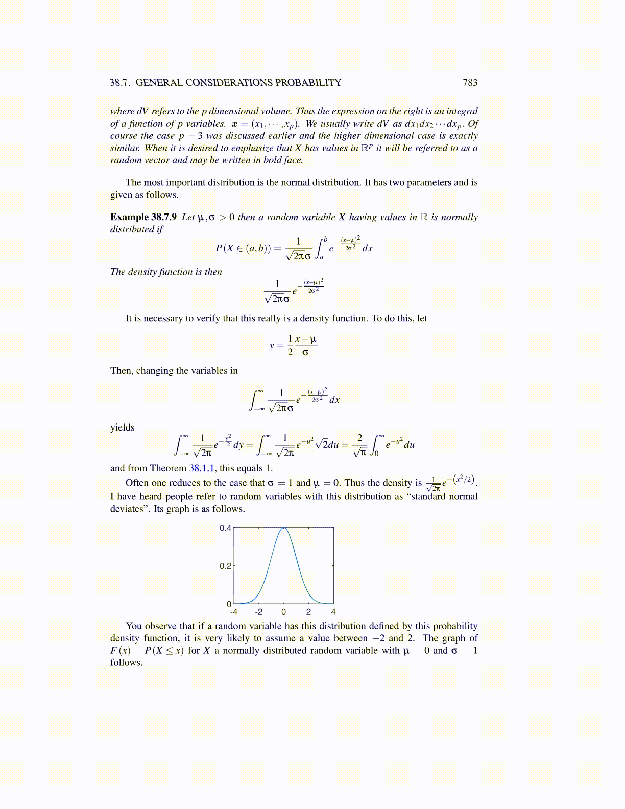
I have heard people refer to random variables with this distribution as “standard normaldeviates”. Its graph is as follows.

-4 -2 0 2 40

0.2

0.4

You observe that if a random variable has this distribution defined by this probabilitydensity function, it is very likely to assume a value between −2 and 2. The graph ofF (x) ≡ P(X ≤ x) for X a normally distributed random variable with µ = 0 and σ = 1follows.