782 CHAPTER 38. PROBABILITY

A modification of this density function gives the very important X 2 (r), chi squared,distribution in the next example.

Example 38.7.7 Let r be a positive integer. The X 2 (r) distribution with r degrees offreedom for a random variable having values in [0,∞) is given by

f (x) =1

Γ(r/2)2r/2 x(r/2)−1e−x/2

Thus there are infinitely many of these, one for each r. I have no idea why they refer to r as“degrees of freedom”.

It is necessary to verify that the above is a probability density. Thus it is necessary toshow that its integral is 1. This involves changing the variable. Let x

2 = t so dx = 2dt then∫∞

0

1Γ(r/2)2r/2 x(r/2)−1e−x/2dx =

∫∞

0

1Γ(r/2)2r/2 (2t)(r/2)−1 e−t2dt

=∫

∞

0

1Γ(r/2)2r/2 2r/2 (t)(r/2)−1 e−tdt = 1

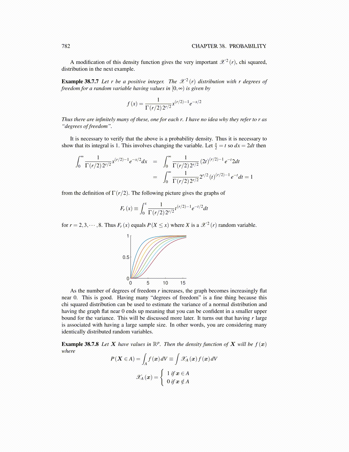
from the definition of Γ(r/2). The following picture gives the graphs of

Fr (x)≡∫ x

0

1Γ(r/2)2r/2 t(r/2)−1e−t/2dt

for r = 2,3, · · · ,8. Thus Fr (x) equals P(X ≤ x) where X is a X 2 (r) random variable.

0 5 10 150

0.5

1

As the number of degrees of freedom r increases, the graph becomes increasingly flatnear 0. This is good. Having many “degrees of freedom” is a fine thing because thischi squared distribution can be used to estimate the variance of a normal distribution andhaving the graph flat near 0 ends up meaning that you can be confident in a smaller upperbound for the variance. This will be discussed more later. It turns out that having r largeis associated with having a large sample size. In other words, you are considering manyidentically distributed random variables.

Example 38.7.8 Let X have values in Rp. Then the density function of X will be f (x)where

P(X ∈ A) =∫

Af (x)dV ≡

∫XA (x) f (x)dV

XA (x) =

{1 if x ∈ A0 if x /∈ A