132 CHAPTER 6. DIRECT SUMS AND BLOCK DIAGONAL MATRICES
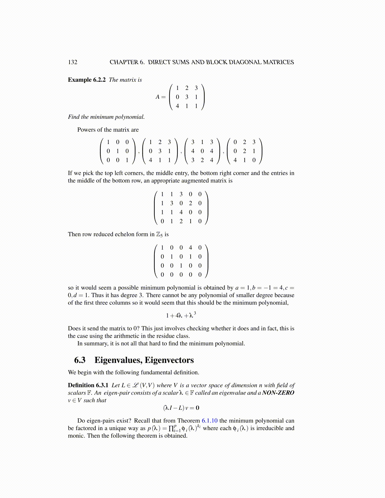
Example 6.2.2 The matrix is
A =
1 2 30 3 14 1 1
Find the minimum polynomial.
Powers of the matrix are 1 0 00 1 00 0 1
,
1 2 30 3 14 1 1
,
3 1 34 0 43 2 4
,
0 2 30 2 14 1 0
If we pick the top left corners, the middle entry, the bottom right corner and the entries inthe middle of the bottom row, an appropriate augmented matrix is
1 1 3 0 01 3 0 2 01 1 4 0 00 1 2 1 0
Then row reduced echelon form in Z5 is
1 0 0 4 00 1 0 1 00 0 1 0 00 0 0 0 0
so it would seem a possible minimum polynomial is obtained by a = 1,b = −1 = 4,c =0,d = 1. Thus it has degree 3. There cannot be any polynomial of smaller degree becauseof the first three columns so it would seem that this should be the minimum polynomial,
1+4λ +λ3
Does it send the matrix to 0? This just involves checking whether it does and in fact, this isthe case using the arithmetic in the residue class.
In summary, it is not all that hard to find the minimum polynomial.
6.3 Eigenvalues, EigenvectorsWe begin with the following fundamental definition.
Definition 6.3.1 Let L ∈L (V,V ) where V is a vector space of dimension n with field ofscalars F. An eigen-pair consists of a scalar λ ∈F called an eigenvalue and a NON-ZEROv ∈V such that
(λ I−L)v = 0
Do eigen-pairs exist? Recall that from Theorem 6.1.10 the minimum polynomial canbe factored in a unique way as p(λ ) = ∏
pi=1 φ i (λ )
ki where each φ i (λ ) is irreducible andmonic. Then the following theorem is obtained.