66 CHAPTER 4. SYSTEMS OF EQUATIONS

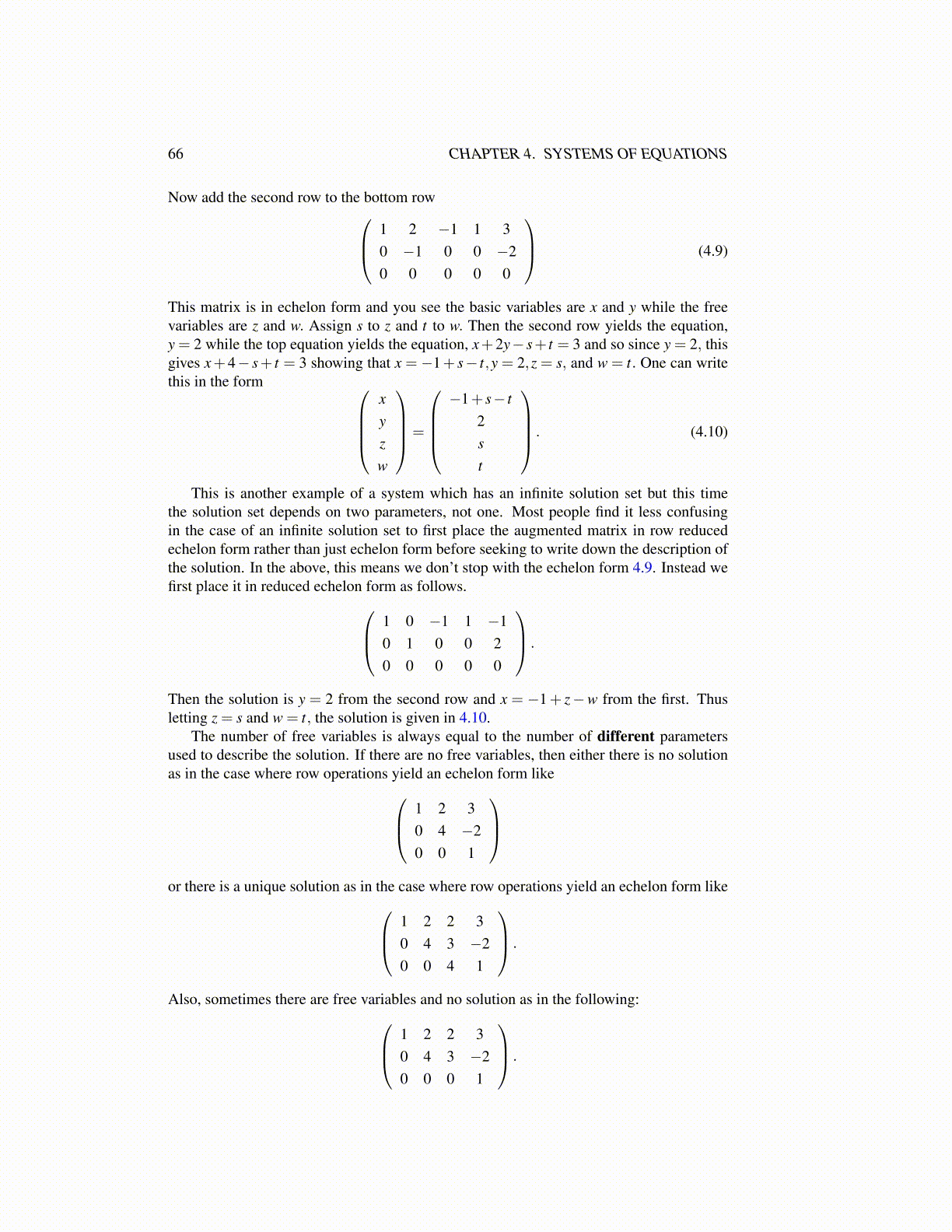
Now add the second row to the bottom row 1 2 −1 1 30 −1 0 0 −20 0 0 0 0

 (4.9)

This matrix is in echelon form and you see the basic variables are x and y while the freevariables are z and w. Assign s to z and t to w. Then the second row yields the equation,y = 2 while the top equation yields the equation, x+2y− s+ t = 3 and so since y = 2, thisgives x+4− s+ t = 3 showing that x =−1+ s− t,y = 2,z = s, and w = t. One can writethis in the form 

xyzw

=

−1+ s− t

2st

 . (4.10)

This is another example of a system which has an infinite solution set but this timethe solution set depends on two parameters, not one. Most people find it less confusingin the case of an infinite solution set to first place the augmented matrix in row reducedechelon form rather than just echelon form before seeking to write down the description ofthe solution. In the above, this means we don’t stop with the echelon form 4.9. Instead wefirst place it in reduced echelon form as follows. 1 0 −1 1 −1

0 1 0 0 20 0 0 0 0

 .

Then the solution is y = 2 from the second row and x = −1+ z−w from the first. Thusletting z = s and w = t, the solution is given in 4.10.

The number of free variables is always equal to the number of different parametersused to describe the solution. If there are no free variables, then either there is no solutionas in the case where row operations yield an echelon form like 1 2 3

0 4 −20 0 1

or there is a unique solution as in the case where row operations yield an echelon form like 1 2 2 3

0 4 3 −20 0 4 1

 .

Also, sometimes there are free variables and no solution as in the following: 1 2 2 30 4 3 −20 0 0 1

 .